Explore picrust2 profile
Source:vignettes/Explore_picrust2_profile.Rmd
Explore_picrust2_profile.RmdFirst, load the rbims package.
The second thing to do would be to read the KO_picrust2_data. The meta file is a tab-separated file containing the name of your ids (bins or sites) and any extra information you would like to use for visualization.
Read metadata
The metadata table can be read in various formats (csv, tsv, txt, xlsx); you will need to use the corresponding function to read the type of file you have. meta and try.
The example data is from an article already published link and were sediment core samples that were collected from three zones of mangrove ecosystem: Basin, Fringe and Impaired. The samples were taken during two seasonal conditions, dry and flood seasons, at three sediment depths: surface (5), mid-layer(20), and deeper sediment layers (40), to assess the impact of degradation level or zone, seasonal variation, and sediment depth on microbial communities.
library(readr)
meta<-read_tsv("../inst/extdata/Metadatos-MANGLAR")
#> Rows: 53 Columns: 10
#> ── Column specification ────────────────────────────────────────────────────────
#> Delimiter: "\t"
#> chr (8): Bin_name, lat, coll_date, ID, seqR2, zone, month, season
#> dbl (2): long, depth
#>
#> ℹ Use `spec()` to retrieve the full column specification for this data.
#> ℹ Specify the column types or set `show_col_types = FALSE` to quiet this message.
head(meta)
#> # A tibble: 6 × 10
#>   Bin_name     lat       long coll_date ID    seqR2     zone  month season depth
#>   <chr>        <chr>    <dbl> <chr>     <chr> <chr>     <chr> <chr> <chr>  <dbl>
#> 1 zr2502_10_R1 18.65135 -91.8 30/5/2018 P10   zr2502_1… Basin May   Dry        5
#> 2 zr2502_43_R1 18.65135 -91.8 30/5/2018 P43   zr2502_4… Basin May   Dry        5
#> 3 zr2502_8_R1  18.65135 -91.8 30/5/2018 P8    zr2502_8… Basin May   Dry        5
#> 4 zr2502_21_R1 18.65135 -91.8 17/1/2018 P21   zr2502_2… Basin Jan   Flood      5
#> 5 zr2502_4_R1  18.65135 -91.8 17/1/2018 P4    zr2502_4… Basin Jan   Flood      5
#> 6 zr2502_5_R1  18.65135 -91.8 17/1/2018 P5    zr2502_5… Basin Jan   Flood      5
Let’s chaghe the names of ids for visualization purposes:
library(dplyr)
#>
#> Attaching package: 'dplyr'
#> The following objects are masked from 'package:stats':
#>
#>     filter, lag
#> The following objects are masked from 'package:base':
#>
#>     intersect, setdiff, setequal, union
library(stringr)
meta <- meta %>%
  mutate(
    Bin_name = str_extract(Bin_name, "(?<=zr2502_)(\\d+)(?=_R1)")
  )
head(meta)
#> # A tibble: 6 × 10
#>   Bin_name lat       long coll_date ID    seqR2        zone  month season depth
#>   <chr>    <chr>    <dbl> <chr>     <chr> <chr>        <chr> <chr> <chr>  <dbl>
#> 1 10       18.65135 -91.8 30/5/2018 P10   zr2502_10_R2 Basin May   Dry        5
#> 2 43       18.65135 -91.8 30/5/2018 P43   zr2502_43_R2 Basin May   Dry        5
#> 3 8        18.65135 -91.8 30/5/2018 P8    zr2502_8_R2  Basin May   Dry        5
#> 4 21       18.65135 -91.8 17/1/2018 P21   zr2502_21_R2 Basin Jan   Flood      5
#> 5 4        18.65135 -91.8 17/1/2018 P4    zr2502_4_R2  Basin Jan   Flood      5
#> 6 5        18.65135 -91.8 17/1/2018 P5    zr2502_5_R2  Basin Jan   Flood      5
Let’s read again the KO_picrust2 data setting profile=F.
KO_picrust2_profile_long <- read_picrust2("../inst/extdata/KO_metagenome_out/KO_pred_metagenome_unstrat.tsv",
                                          database = "KO",
                                          profile = F)
head(KO_picrust2_profile_long)
#> # A tibble: 6 × 3
#>   KO     Bin_name     Abundance
#>   <chr>  <chr>            <dbl>
#> 1 K00001 zr2502_1_R1         82
#> 2 K00001 zr2502_10_R1       407
#> 3 K00001 zr2502_11_R1         0
#> 4 K00001 zr2502_12_R1       243
#> 5 K00001 zr2502_13_R1         0
#> 6 K00001 zr2502_14_R1       184
The same change in Bin names:
KO_picrust2_profile_long <- KO_picrust2_profile_long %>%
  mutate(
    Bin_name = str_extract(Bin_name, "(?<=zr2502_)(\\d+)(?=_R1)")
  )
head(KO_picrust2_profile_long)
#> # A tibble: 6 × 3
#>   KO     Bin_name Abundance
#>   <chr>  <chr>        <dbl>
#> 1 K00001 1               82
#> 2 K00001 10             407
#> 3 K00001 11               0
#> 4 K00001 12             243
#> 5 K00001 13               0
#> 6 K00001 14             184
Map to the KEGG database
Then map the KO to the rest of the features of the KEGG and rbims database.
ko_bin_mapp<-mapping_ko(KO_picrust2_profile_long)Metabolism subsetting
In this example, we will use energy metabolism to explore the rest of the functions.
- Create a vector with the metabolism of interest.
Other_energy<-c("Fermentation", "Carbon fixation", "Methane metabolism",
"Sulfur metabolism", "Nitrogen metabolism")- Use get_subset_pathway to subset the table using the cycles and the information of the energy metabolism.
library(tidyr)
Energy_metabolisms<-ko_bin_mapp %>%
  drop_na(Cycle, Pathway_cycle) %>%
get_subset_pathway(Cycle, Other_energy)- Plot the information using the plot_heatmap function. The argument order_y will order the rows according to a metabolic feature; in this case, we order the pathways_cycle according to cycle.
plot_heatmap(tibble_ko=Energy_metabolisms,
             y_axis=Pathway_cycle,
             order_y = Cycle,
             split_y = TRUE,
            data_experiment = meta,
             order_x = "zone",
             analysis = "KEGG",
             calc="Percentage")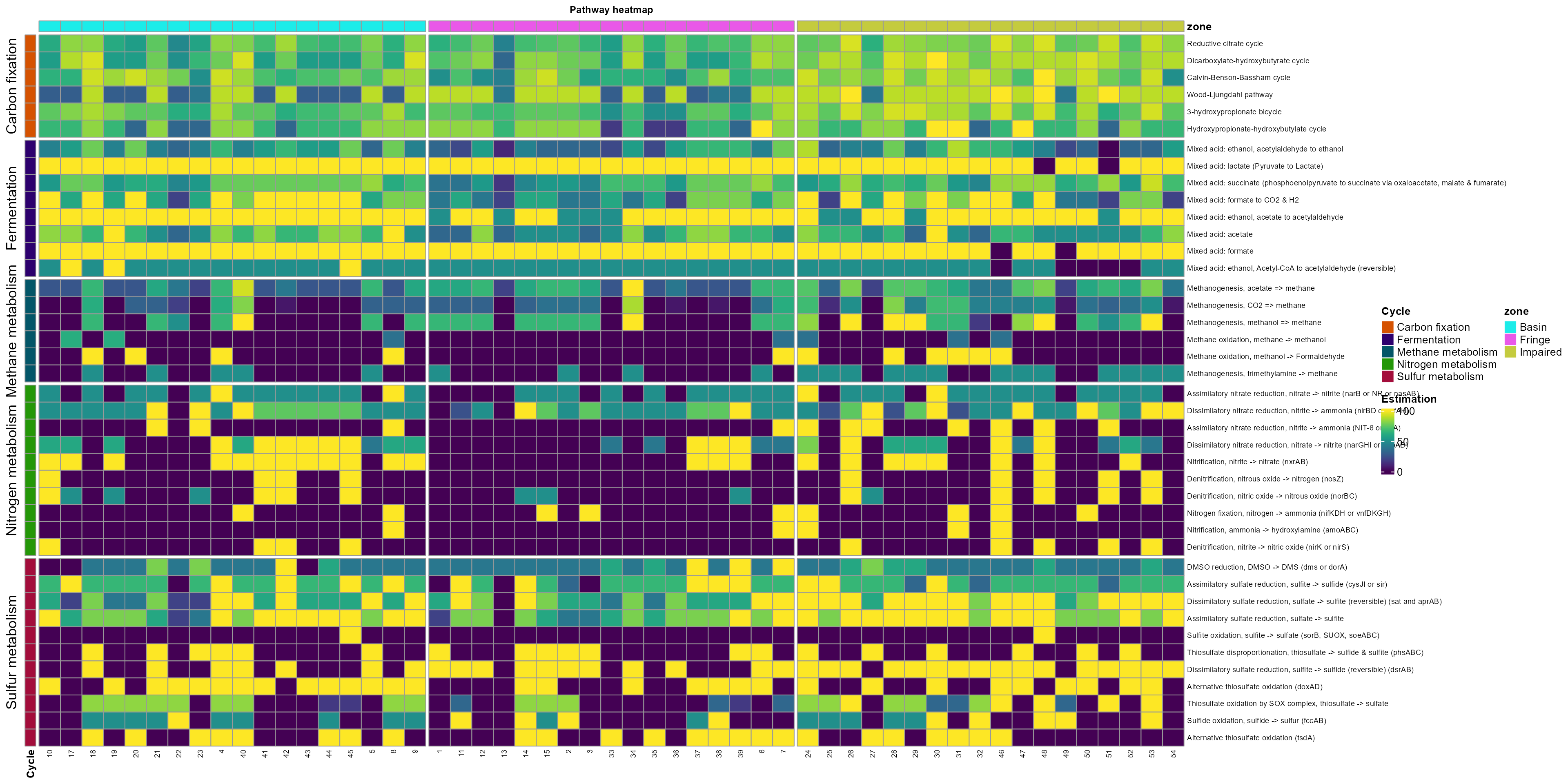
Example of exploring a specific KEGG pathway
specific<-c("map05416", "map00363", "map00604", "map00908", "map00941")- Now, let’s extract the profile associated with that metabolic pathway.
library(tidyr)
specific_subset<-ko_bin_mapp%>%
  drop_na(Pathway) %>%
  get_subset_pathway(Pathway, specific)
head(specific_subset)
#> # A tibble: 5 × 66
#>   Module Module_description      Pathway Pathway_description Cycle Pathway_cycle
#>   <chr>  <chr>                   <chr>   <chr>               <chr> <chr>
#> 1 M00039 Monolignol biosynthesi… map009… Flavonoid biosynth… NA    NA
#> 2 NA     NA                      map009… Zeatin biosynthesis NA    NA
#> 3 NA     NA                      map054… Viral myocarditis   NA    NA
#> 4 M00079 Keratan sulfate degrad… map006… Glycosphingolipid … NA    NA
#> 5 NA     NA                      map003… Bisphenol degradat… NA    NA
#> # ℹ 60 more variables: Detail_cycle <chr>, Genes <chr>, Gene_description <chr>,
#> #   Enzyme <chr>, KO <chr>, rbims_pathway <chr>, rbims_sub_pathway <chr>,
#> #   `1` <dbl>, `10` <dbl>, `11` <dbl>, `12` <dbl>, `13` <dbl>, `14` <dbl>,
#> #   `15` <dbl>, `17` <dbl>, `18` <dbl>, `19` <dbl>, `2` <dbl>, `20` <dbl>,
#> #   `21` <dbl>, `22` <dbl>, `23` <dbl>, `24` <dbl>, `25` <dbl>, `26` <dbl>,
#> #   `27` <dbl>, `28` <dbl>, `29` <dbl>, `3` <dbl>, `30` <dbl>, `31` <dbl>,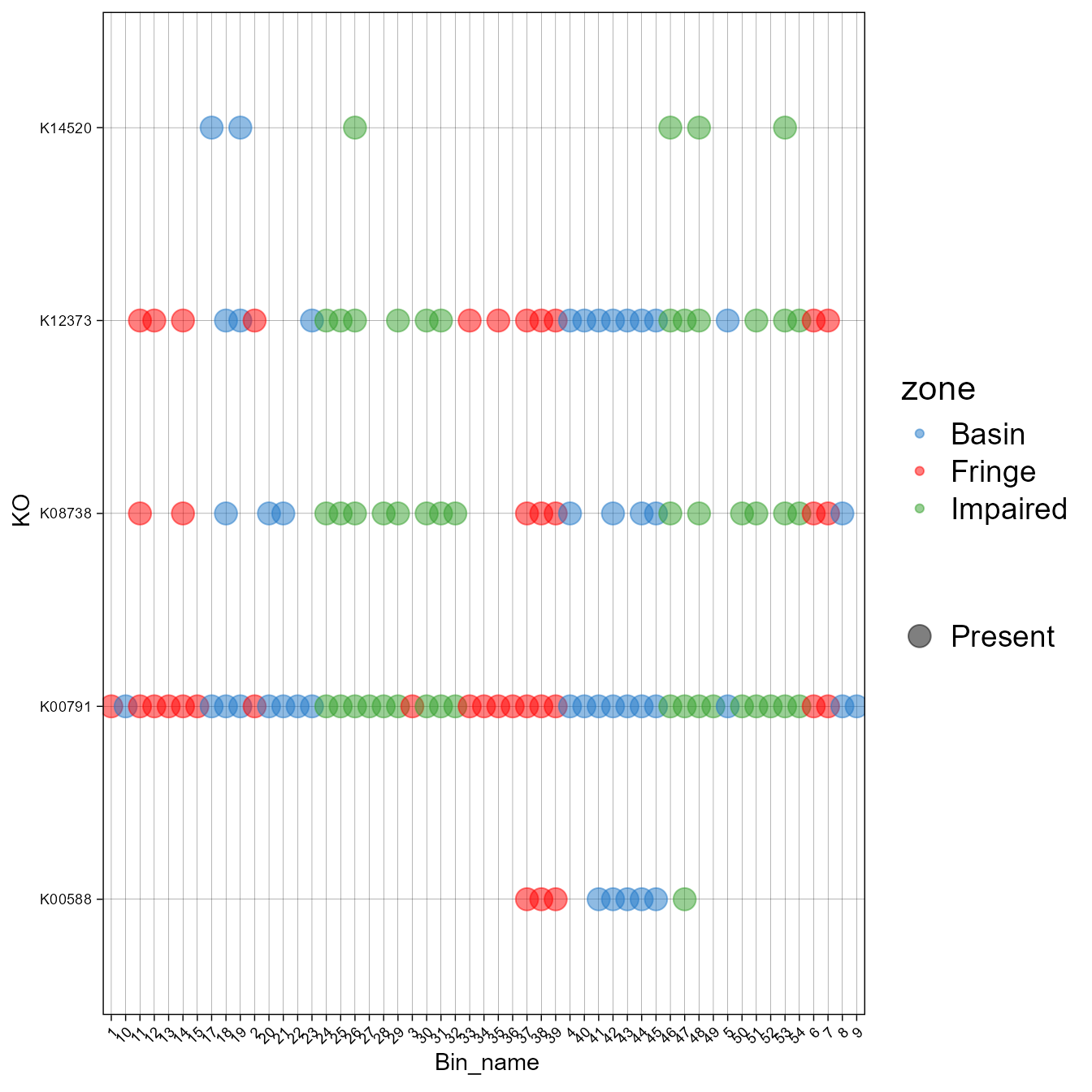
#> # `32` <dbl>, `33` <dbl>, `34` <dbl>, `35` <dbl>, `36` <dbl>, `37` <dbl>, …- Now, let’s create a plot of the presence and absence of the different KO associated with that pathway. Besides presence and absence, it is possible to plot abundance or the percentage of genes within certain pathways (See plot_bubble, calc argument).
plot_bubble(tibble_ko = specific_subset,
            x_axis = Bin_name,
            y_axis = KO,
            analysis="KEGG",
            data_experiment = meta,
            color_character = zone,
            calc="Binary",
            range_size = c(1,10))