Explore merops profile

library(rbims)

Let’s load the merops data:

merops_profile <- read_merops("../inst/extdata/peptidase_2/", 
                              profile = T)

For MEROPS the functions plot_heatmap and plot_bubble can be used as well as the other data.

Let’s choose the top 10 most abundant pathways:

library(tidyverse)
merops_profile_100 <- merops_profile %>% mutate(
    avg = rowMeans(across(where(is.numeric)), na.rm = TRUE)) %>% top_n(100,avg) %>% dplyr::select(-avg)

The bubble plot:

plot_bubble(merops_profile_100,
            y_axis = MEROPS_family,
            range_size= c(0,1.5),
            x_axis= Bin_name,
            analysis = "MEROPS",
            calc = "Binary")
#> Scale for size is already present.
#> Adding another scale for size, which will replace the existing scale.
#> Warning: Removed 548 rows containing missing values or values outside the scale range
#> (`geom_point()`).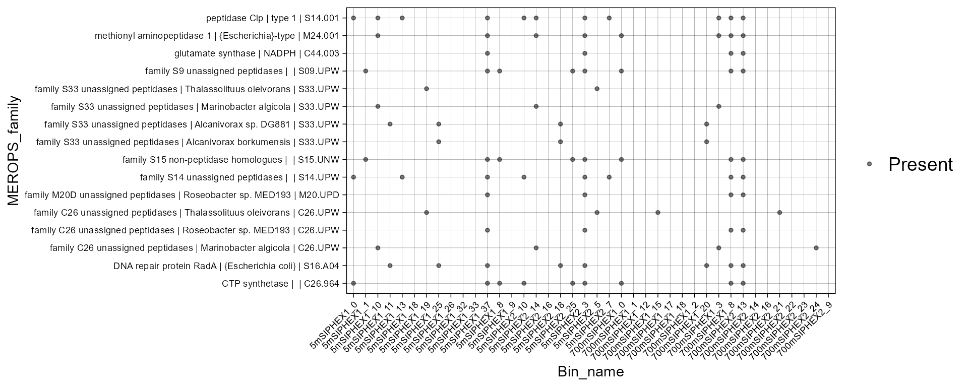

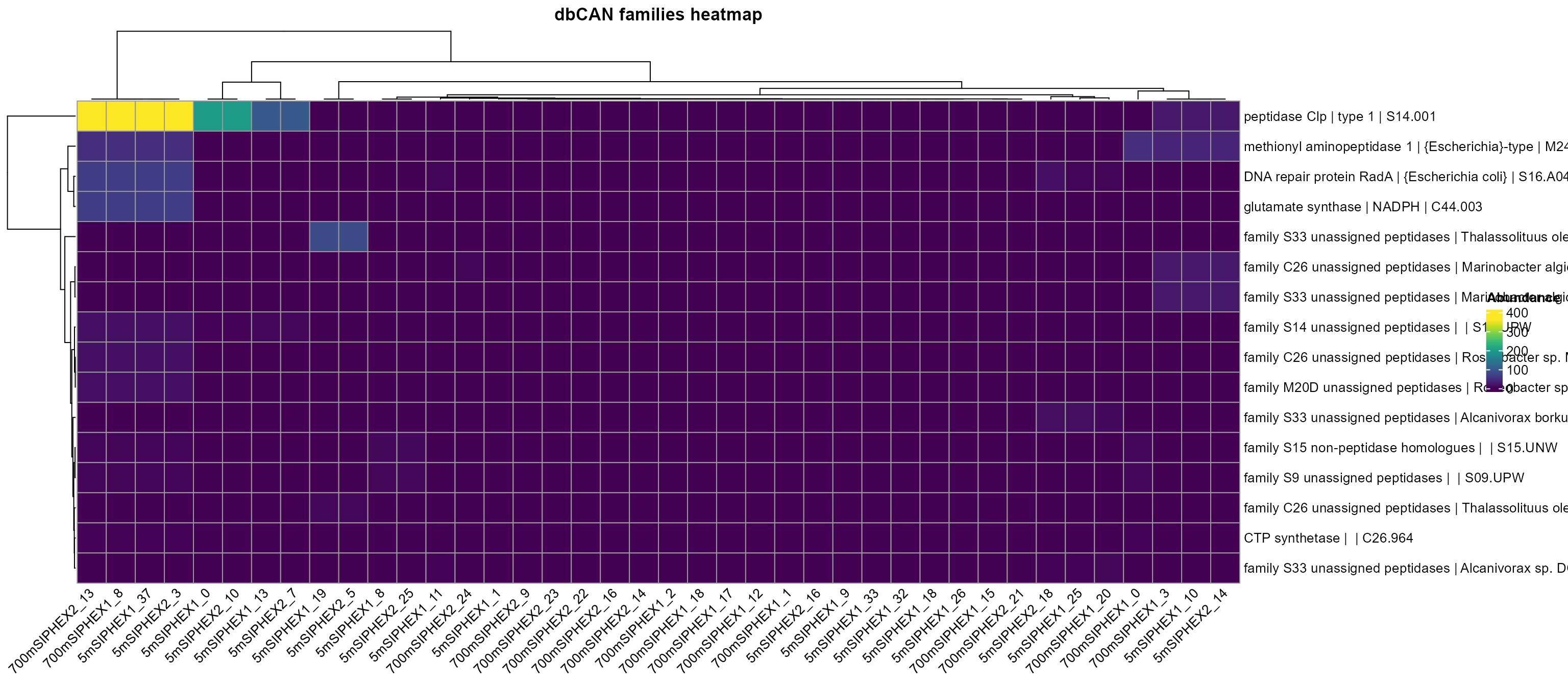
Now let’s group for avoiding repetitions in row.names for heatmap:

merops_profile_100_distinct <- merops_profile_100 %>%   group_by(MEROPS_family) %>%
  summarise(
    domain_name = first(domain_name),  
    across(where(is.numeric), sum)
  )

plot_heatmap(
  merops_profile_100_distinct,
  y_axis = MEROPS_family,
  analysis = "MEROPS",
  distance = F
)
#> Warning: The input is a data frame, convert it to the matrix.