Explore dbcan profile

library(rbims)

Let’s load the dbcan3 data:

dbcan_profile <-read_dbcan3(dbcan_path = "../inst/extdata/test_data/", 
                            profile = T, 
                            write = F)
#> Warning: Expected 1 pieces. Additional pieces discarded in 12 rows [1, 2, 3, 7, 9, 13,
#> 16, 17, 22, 24, 31, 36].
#> Warning: Expected 1 pieces. Additional pieces discarded in 44 rows [1, 2, 3, 4, 5, 6, 7,
#> 8, 9, 10, 11, 12, 13, 14, 15, 16, 17, 18, 19, 20, ...].
#> [1] "Input Genes = 123"
#> [1] "Remained Genes after filtering = 44"
#> [1] "Percentage of genes remained = 36%"
#> [1] "Number of genes with signals = 2"
#> [1] "Number of genes with signals that passed filtering = 2"

For dbCAN the functions plot_heatmap and plot_bubble can be used as well.

plot_heatmap(dbcan_profile, 
             y_axis=dbCAN_family, 
             analysis = "dbCAN", 
             distance = T)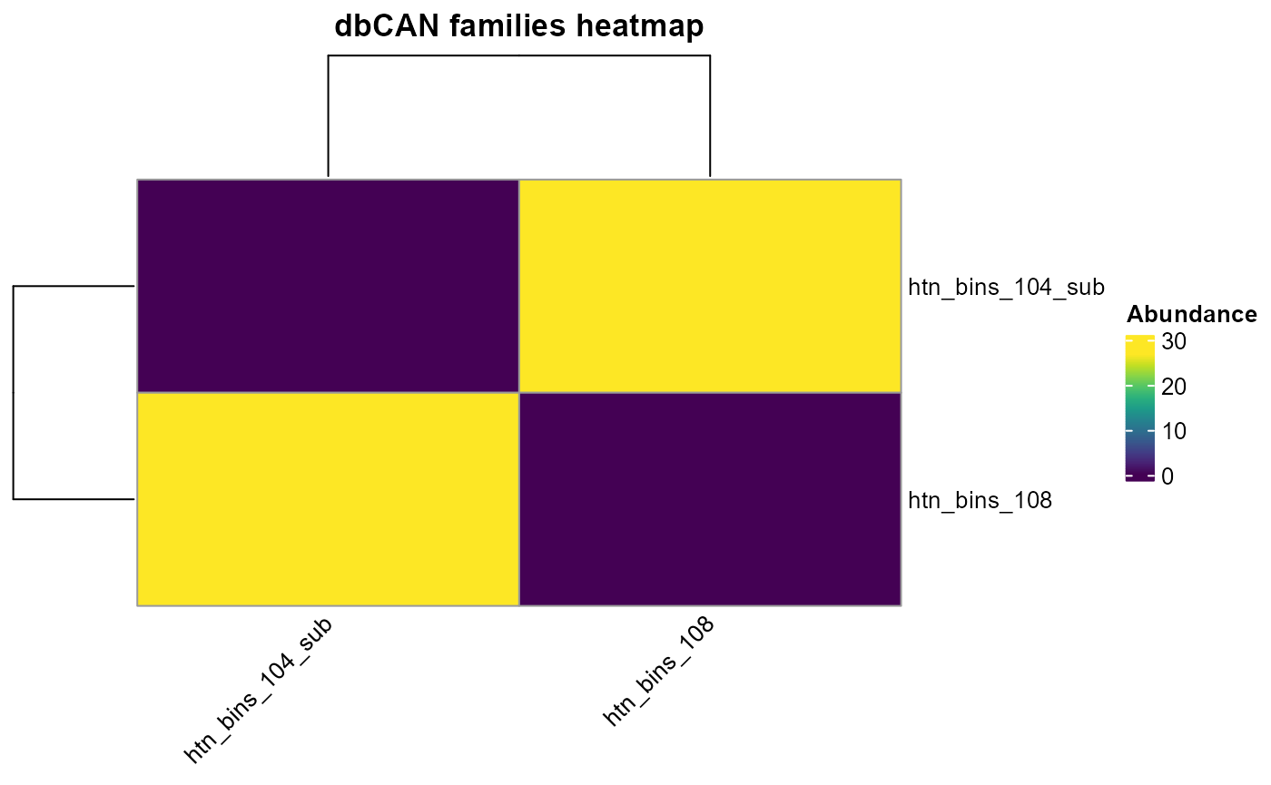

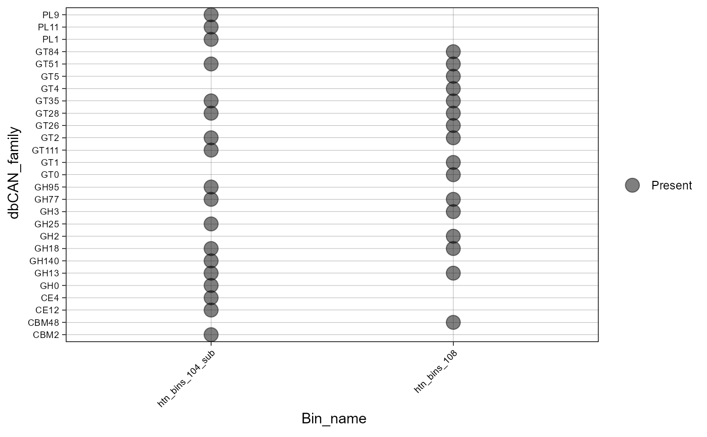
plot_bubble(dbcan_profile, 
            y_axis=dbCAN_family, 
            x_axis=Bin_name, 
            calc = "Binary",
            analysis = "dbCAN")
#> Warning: Removed 20 rows containing missing values or values outside the scale range
#> (`geom_point()`).