13. Discriminant analysis and pathway-level directional bias in RBIMS
RBIMS
Source:vignettes/13_Discriminant_analysis.Rmd
13_Discriminant_analysis.Rmd1. Overview
This vignette demonstrates how to:
- Run KO-level discriminant analysis using
get_subset_discriminant(). - Inspect consensus statistics and effect sizes.
- Visualize discriminant features.
- Quantify pathway-level directional bias using a binomial framework.
The goal is to move from feature-level statistics to ecologically interpretable pathway-level patterns.
2. Required data structure
The KO table must:
- Contain a feature column (e.g.,
"KO"). - Contain numeric columns corresponding to MAG abundances.
- Optionally include annotation columns such as
rbims_pathway.
The metadata must:
- Contain a
Bin_namecolumn matching MAG column names. - Contain a grouping variable (e.g.,
"Depth").
3. Load libraries
library(rbims)
library(dplyr)
#>
#> Attaching package: 'dplyr'
#> The following objects are masked from 'package:stats':
#>
#>     filter, lag
#> The following objects are masked from 'package:base':
#>
#>     intersect, setdiff, setequal, union
library(tidyr)
library(tibble)
library(ggplot2)
library(forcats)
4. Sanity checks
stopifnot("KO" %in% names(ko_table))

mag_cols <- ko_table %>%
  select(where(is.numeric)) %>%
  names()

stopifnot(length(mag_cols) > 1)

stopifnot(all(c("Bin_name", "Depth") %in% names(metadata)))

metadata_use <- metadata %>%
  select(Bin_name, Depth)

stopifnot(all(mag_cols %in% metadata_use$Bin_name))
stopifnot(nlevels(factor(metadata_use$Depth)) == 2)
5. Run discriminant analysis
tibble_disc <- get_subset_discriminant(
  tibble_rbims = ko_table,
  metadata     = metadata_use,
  analysis     = "KEGG",
  group_col    = "Depth",
  feature_col  = "KO",
  min_presence = 3,
  score_min    = 1
)

disc_obj <- attr(tibble_disc, "rbims_disc")
Inspect score distribution:
6. Visualizing discriminant features
6.1 Heatmap (Depth × Feature)
plot_disc_heatmap(
  disc_obj  = disc_obj,
  metadata  = metadata_use,
  group_col = "Depth",
  top_n     = 40
)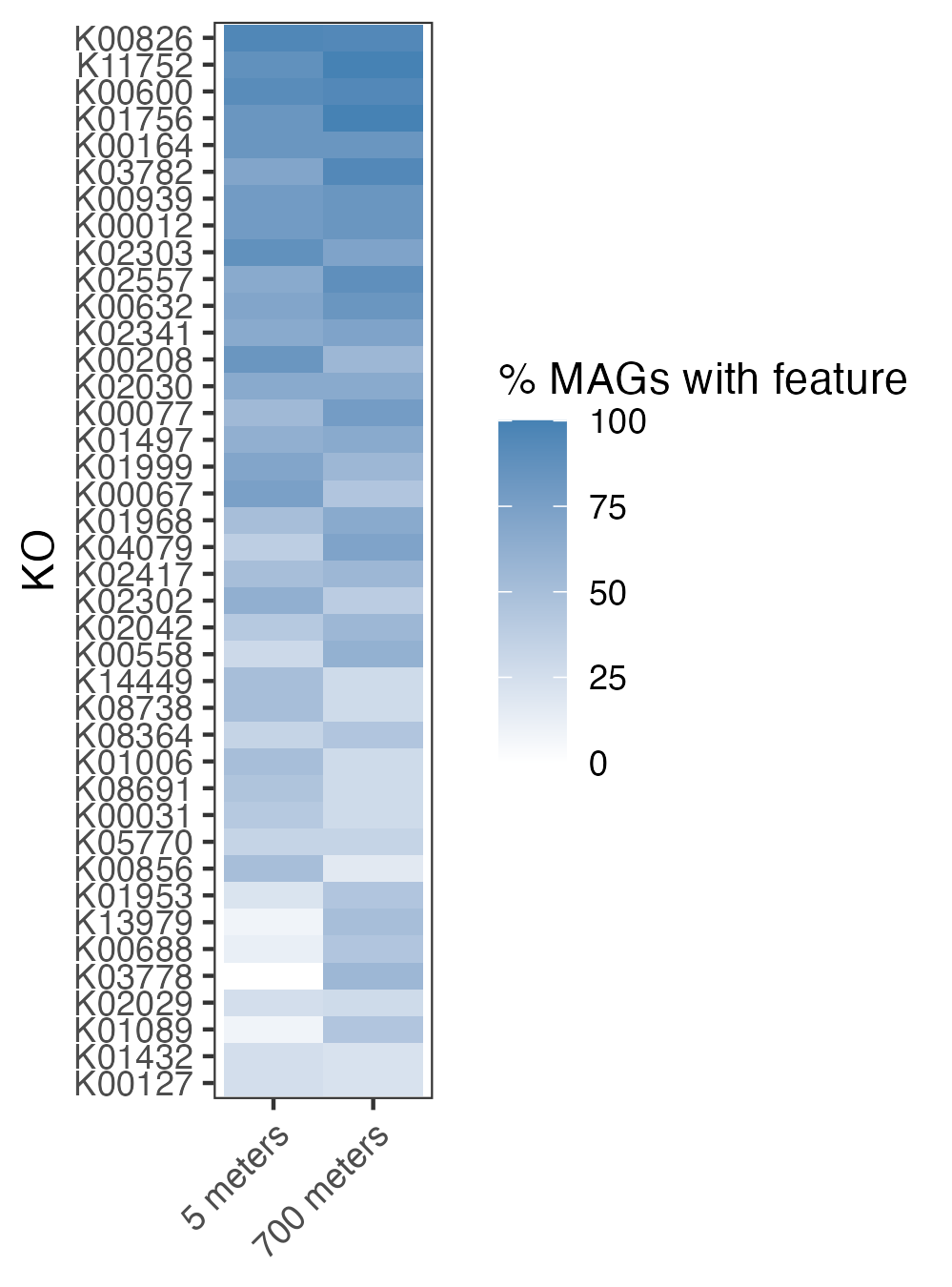
Figure 1: The top 20 enriched KOs and their
coverage per sampling environment
6.2 Effect size plot
plot_disc_effect(disc_obj, top_n = 40)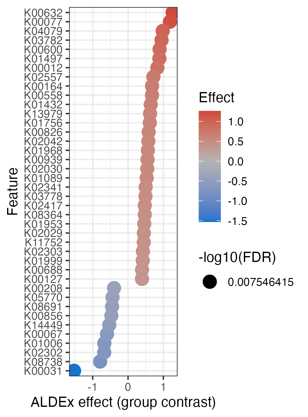
Figure 2: Effect size of the ALDEx analysis,
showcasing that the top 3 KOs are the most abundant in the MAGs from
deep environments (effect > 1)
7. Pathway-level directional bias
7.1 Build KO dictionary
ko_dictionary <- make_ko_dictionary(
  tibble_rbims = ko_table,
  feature_col  = "KO"
)
7.2 Calculate pathway-level directional bias
pathways <- c("Hexadecane", "Naphthalene", "Phenanthrene")

pathway_tbl <- calc_pathway_directional_bias(
  disc_obj      = disc_obj,
  ko_dictionary = ko_dictionary,
  pathways      = pathways,
  p_null        = 0.5,
  p_alternative = "greater",
  ci_two_sided  = TRUE
)

pathway_tbl
7.3 Visualize pathway-level bias
plot_pathway_directional_bias(
  pathway_tbl,
  reorder = TRUE,
  show_fdr_label = TRUE
)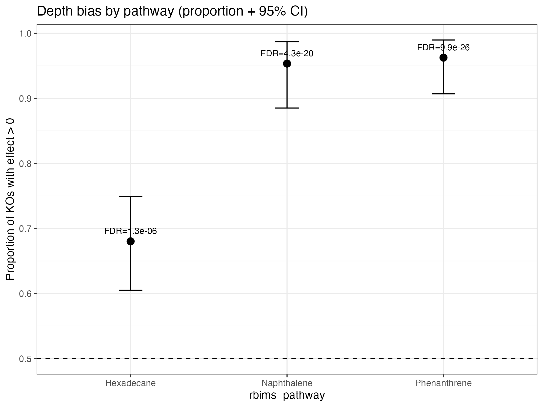
Figure 3: Proportion of KEGG Orthologs (KOs)
within each pathway showing positive discriminant effect values (effect
> 0)
8. Interpretation
A pathway shows directional bias when:
- A large fraction of its KOs share the same effect direction.
- The binomial test indicates the proportion exceeds 0.5.
- The result remains significant after FDR correction.